For memory, identifying memory bandwidth is quite straightforward, as the three types of memory—SDRAM, DDR, and RDRAM—are visually distinct. The main thing to recognize is the different frequencies of DDR memory.
With the continuous advancement of deep learning, computing power has become a major focus within the community. At the end of the day, every deep learning model must run on a device, and the lower the model's requirements for hardware performance, the more applications it can support. It’s essential not to let hardware become the bottleneck of the model!
When considering the hardware requirements of a model, the first thing that comes to mind is the amount of computation—how many operations a model needs to perform during a single forward pass. However, in addition to computation, the model’s demand for memory bandwidth is also a critical factor that influences actual execution time. As we’ll see below, even reducing the number of computations doesn’t always lead to a proportional decrease in runtime when memory bandwidth is limited.

The impact of memory bandwidth on system performance is illustrated above. If we compare memory to a bottle and the processing unit to a cup, data becomes the particles inside the bottle, and the memory interface is the mouth of the bottle. Data can be consumed (processed) through this opening. Memory bandwidth represents the width of the bottle’s mouth. The narrower the mouth, the longer it takes for data to flow into the cup (processing unit). In other words, if the bandwidth is limited, even with an extremely fast processing unit, it often ends up idle while waiting for data, leading to wasted computing power.
Deep Learning Networks and the Roofline ModelFor engineers, qualitative analysis isn't enough. We also need to be able to quantitatively evaluate how much memory bandwidth a model requires and how it affects computing performance.
The requirement for memory bandwidth is typically expressed using operand intensity (or arithmetic intensity), measured in operations per byte (OPs/byte). This value indicates how many operations can be supported per unit of data read. The higher the intensity, the fewer memory bandwidth demands the algorithm has, which is ideal for performance.
Let’s take an example: consider a 3x3 convolution with a stride of 1, where the input size is 64x64. Assuming both input and output features are 1, there are 62x62 convolutions, each requiring 9 multiply-add operations. That totals 34,596 operations. The data size would be 64x64x2 (input) + 3x3x2 (kernel) = 8,210 bytes. So the intensity is 34,596 / 8,210 ≈ 4.21. Now, if we switch to a 1x1 convolution, the total operations drop to 64x64 = 4,096, but the data size is 64x64x2 + 1x1x2 = 8,194 bytes. The intensity then drops to 0.5, meaning the memory bandwidth demand increases by 9 times. If the bandwidth is insufficient, the 1x1 convolution may actually run slower than the 3x3 one, despite having less computation.
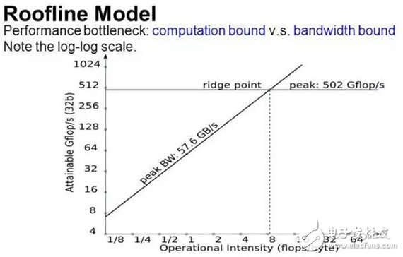
This shows that deep learning systems face two main bottlenecks: computing power and memory bandwidth. To determine which limits performance, the Roofline model is useful.
The typical Roofline curve is shown above. The vertical axis represents computational performance, and the horizontal axis represents computational intensity. The curve splits into two regions: a rising slope on the left and a flat region on the right. When the algorithm’s intensity is low, performance is constrained by memory bandwidth, and many computing units remain idle. As intensity increases, more operations can be performed per unit of data, leading to better utilization and higher performance. Eventually, all units are used, and the curve enters the saturation region, where performance is limited by computing power rather than memory bandwidth.
Clearly, if memory bandwidth is very wide, algorithms don’t need to be highly intensive to hit the performance ceiling set by computing power. As shown in the next figure, increasing memory bandwidth lowers the intensity required to reach that ceiling.
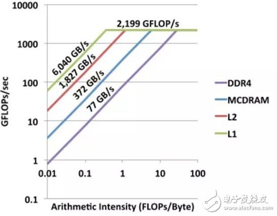
The Roofline model is crucial for algorithm-hardware co-design, helping us decide whether to increase memory bandwidth, reduce memory requirements, or boost computing power. If the algorithm is in the rising region, improving memory bandwidth or reducing memory usage is more effective than just increasing compute power. Conversely, if it's in the saturation region, boosting computing power becomes the priority.
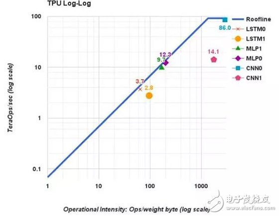
Let’s look at a real-world example: the location of various machine learning algorithms on the Roofline model. From Google’s TPU paper, we see that LSTM has the lowest computational intensity, placing it in the rising region. As a result, its performance on TPU is only about 3 TOPS, far below the peak of 90 TOPS. MLP has slightly better intensity but still remains in the rising region, achieving around 10 TOPS. Convolutional neural networks, especially CNN0, have high intensity and approach the TPU’s roofline (86 TOPS). However, CNN1, though intense, doesn’t reach the top due to other factors like shallow feature depth. This highlights another important point: besides memory bandwidth, there are other factors that might prevent an algorithm from reaching its full potential. We should aim to minimize these “other factors†as much as possible.
Lithium Battery Cr9V,Lithium Battery 9V,9V Lithium Battery,9V Lithium Battery Pack
Jiangmen Hongli Energy Co.ltd , https://www.honglienergy.com